2. Huang Example

Let’s go over the Huang Bayesian Belief Network (BBN) [HD99].

2.1. Model

The Huang BBN is stored in a JSON file. For completeness, we show the content of the JSON file.

import json

with open('../../_support/bbn/huang-bbn.json', 'r') as fp:
    data = json.load(fp)

data

{'d': {'nodes': ['A', 'B', 'C', 'D', 'E', 'F', 'G', 'H'],
  'edges': [['A', 'B'],
   ['A', 'C'],
   ['B', 'D'],
   ['C', 'E'],
   ['C', 'G'],
   ['D', 'F'],
   ['E', 'F'],
   ['E', 'H'],
   ['G', 'H']]},
 'p': {'A': {'columns': ['A', '__p__'], 'data': [['on', 0.5], ['off', 0.5]]},
  'B': {'columns': ['A', 'B', '__p__'],
   'data': [['on', 'on', 0.5],
    ['on', 'off', 0.5],
    ['off', 'on', 0.4],
    ['off', 'off', 0.6]]},
  'C': {'columns': ['A', 'C', '__p__'],
   'data': [['on', 'on', 0.7],
    ['on', 'off', 0.3],
    ['off', 'on', 0.2],
    ['off', 'off', 0.8]]},
  'D': {'columns': ['B', 'D', '__p__'],
   'data': [['on', 'on', 0.9],
    ['on', 'off', 0.1],
    ['off', 'on', 0.5],
    ['off', 'off', 0.5]]},
  'E': {'columns': ['C', 'E', '__p__'],
   'data': [['on', 'on', 0.3],
    ['on', 'off', 0.7],
    ['off', 'on', 0.6],
    ['off', 'off', 0.4]]},
  'F': {'columns': ['D', 'E', 'F', '__p__'],
   'data': [['on', 'on', 'on', 0.01],
    ['on', 'on', 'off', 0.99],
    ['on', 'off', 'on', 0.01],
    ['on', 'off', 'off', 0.99],
    ['off', 'on', 'on', 0.01],
    ['off', 'on', 'off', 0.99],
    ['off', 'off', 'on', 0.99],
    ['off', 'off', 'off', 0.01]]},
  'G': {'columns': ['C', 'G', '__p__'],
   'data': [['on', 'on', 0.8],
    ['on', 'off', 0.2],
    ['off', 'on', 0.1],
    ['off', 'off', 0.9]]},
  'H': {'columns': ['E', 'G', 'H', '__p__'],
   'data': [['on', 'on', 'on', 0.05],
    ['on', 'on', 'off', 0.95],
    ['on', 'off', 'on', 0.95],
    ['on', 'off', 'off', 0.05],
    ['off', 'on', 'on', 0.95],
    ['off', 'on', 'off', 0.05],
    ['off', 'off', 'on', 0.95],
    ['off', 'off', 'off', 0.05]]}}}

From this BBN-specified JSON file, we will create the capable reasoning model.

from pybbn.factory import create_reasoning_model

model = create_reasoning_model(data['d'], data['p'])

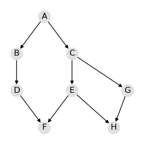
2.1.1. Graph (DAG)

We can visualize the directed acyclic graph (DAG) of the Huang BBN.

from help.viz import *

draw_dag(model)

2.1.2. Parameters

Here are the parameters of the Huang BBN.

model.node_potentials['A']

	A	__p__
0	on	0.5
1	off	0.5

model.node_potentials['B']

	A	B	__p__
0	on	on	0.5
1	on	off	0.5
2	off	on	0.4
3	off	off	0.6

model.node_potentials['C']

	A	C	__p__
0	on	on	0.7
1	on	off	0.3
2	off	on	0.2
3	off	off	0.8

model.node_potentials['D']

	B	D	__p__
0	on	on	0.9
1	on	off	0.1
2	off	on	0.5
3	off	off	0.5

model.node_potentials['E']

	C	E	__p__
0	on	on	0.3
1	on	off	0.7
2	off	on	0.6
3	off	off	0.4

model.node_potentials['F']

	D	E	F	__p__
0	on	on	on	0.01
1	on	on	off	0.99
2	on	off	on	0.01
3	on	off	off	0.99
4	off	on	on	0.01
5	off	on	off	0.99
6	off	off	on	0.99
7	off	off	off	0.01

model.node_potentials['G']

	C	G	__p__
0	on	on	0.8
1	on	off	0.2
2	off	on	0.1
3	off	off	0.9

model.node_potentials['H']

	E	G	H	__p__
0	on	on	on	0.05
1	on	on	off	0.95
2	on	off	on	0.95
3	on	off	off	0.05
4	off	on	on	0.95
5	off	on	off	0.05
6	off	off	on	0.95
7	off	off	off	0.05

2.2. Graphs

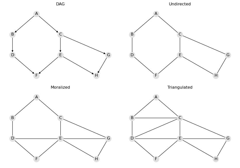
2.2.1. Intermediate graphs

It might be interesting to see the intermediate graphs created. Here’s what the graphs below represent.

• DAG: the Huang DAG associated with the Huang BBN

• Undirected: the undirected graph of the Huang DAG (directed edges are removed)

• Moralized: the moralized graph of the Huang DAG

• Triangulated: the triangulated graph of the Huang DAG

draw_intermediate_graphs(model)

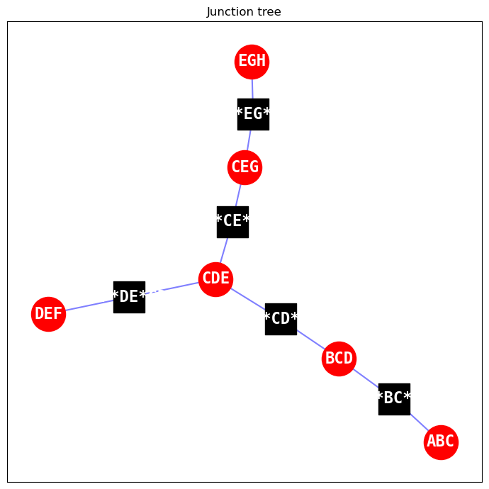
2.2.2. Join tree

The join tree is the main inferencing engine of the reasoning model. We can choose to visualize the join tree too.

• red nodes: these are the cliques/clusters of the join tree

• black nodes: these are the separation sets of the join tree

draw_junction_tree(model)

2.3. Queries

Queries can be classified as follows.

• Marginal query (univariate probabilities)

• Associational query (conditional probabilities)

• Interventional query (causal effect probabilities)

• Counterfactual query (counterfactual probabilities)

The above categories of queries follow Pearl’s Causal Hierarchy (PCH) or the Causal Ladder [GDH22].

2.3.1. Marginal query

Let’s just follow one variable, \(H\). The marginal probability of \(H\), \(P(H)\), is easy to query.

q = model.pquery()
q['H']

	H	__p__
0	off	0.1769
1	on	0.8231

2.3.2. Associational query

In an associational query, we want to compute the conditional probabilities

• \(P(H|E=\mathrm{on})\), and

• \(P(H|E=\mathrm{off})\).

q = model.pquery(evidences=model.e({'E': 'on'}))
q['H']

	H	__p__
0	off	0.322903
1	on	0.677097

q = model.pquery(evidences=model.e({'E': 'off'}))
q['H']

	H	__p__
0	off	0.05
1	on	0.95

2.3.3. Interventional query

The interventional query is estimating the causal effect one one variable on another. In this case, we want to estimate the causal effect of \(E\) on \(H\). However, \(E\) and \(H\) are confounded through \(\{C, G\}\). We need to apply the do-operator on \(E\) to estimate the causal effect of \(E\) on \(H\). (The causal effect of \(E\) on \(H\) is not simply the associational query we performed above!)

\(P(H=h|\mathrm{do}(E=e))\)

We do not have to control for both counfounders \(\{C, G\}\), it is sufficient to just control for \(C\) to block backdoor paths from \(E\) to \(H\). Thus, using the backdoor adjustment formula, we can compute the causal effect as follows.

\(P(H=h|\mathrm{do}(E=e)) = \sum_C P(H=h|E=e, C)P(C)\)

Let’s compute two causal effects.

• \(P(H=\mathrm{on}|\mathrm{do}(E=\mathrm{on})) = \sum_C P(H=\mathrm{on}|E=\mathrm{on}, C)P(C)\)

• \(P(H=\mathrm{on}|\mathrm{do}(E=\mathrm{off})) = \sum_C P(H=\mathrm{on}|E=\mathrm{off}, C)P(C)\)

p_on = model.iquery(Y=['H'], y=['on'], X=['E'], x=['on'])
p_on

H    0.5765
dtype: float64

p_off = model.iquery(Y=['H'], y=['on'], X=['E'], x=['off'])
p_off

H    0.95
dtype: float64

The average causal effect (ACE) is defined as follows.

\(\mathrm{ACE} = P(H=\mathrm{on}|\mathrm{do}(E=\mathrm{on})) - P(H=\mathrm{on}|\mathrm{do}(E=\mathrm{off}))\)

p_on['H'] - p_off['H']

-0.37349999999999994

2.3.4. Counterfactual query

In this counterfactual query, we have the following.

• query: \(H\)

• factual: \(E=\mathrm{on}, G=\mathrm{on}, H=\mathrm{on}\)

• counterfactual: \(E=\mathrm{off}\)

The query is against \(H\); it is the variable we are interested in. The factual is what actually happened. The counterfactual is the hypothetical. Let’s try to word this as a counterfactual statement (not so easy to do).

• Given that \(E\) was on, \(G\) was on, \(H\) was on, what is the probability of \(H\) had we set \(E\) to off?

Y = 'H'
e = {
    'E': 'on',
    'G': 'on',
    'H': 'on'
}
h = {
    'E': 'off'
}
model.cquery(Y, e, h)

	H	__p__
0	off	0.043749
1	on	0.956251

Let’s try another counterfactual query. We have the following.

• query: \(H\)

• factual: \(E=\mathrm{off}, G=\mathrm{off}, H=\mathrm{off}\)

• counterfactual: \(E=\mathrm{on}\)

As a counterfactual statement, we might naturally say the following (?).

• Given that \(E\) was off, \(G\) was off, \(H\) was off, what is the probability of \(H\) had we set \(E\) to on?

Y = 'H'
e = {
    'E': 'off',
    'G': 'off',
    'H': 'off'
}
h = {
    'E': 'on'
}
model.cquery(Y, e, h)

	H	__p__
0	off	0.439756
1	on	0.560244

Here’s the last counterfactual query. We have the following.

• query: \(H\)

• factual: \(E=\mathrm{on}, G=\mathrm{on}, H=\mathrm{on}\)

• counterfactual: \(E=\mathrm{off}, G=\mathrm{off}\)

As a counterfactual statement, we might naturally say the following (?).

• Given that \(E\) was on, \(G\) was on, \(H\) was on, what is the probability of \(H\) had we set \(E\) and \(G\) to off?

Y = 'H'
e = {
    'E': 'on',
    'G': 'on',
    'H': 'on'
}
h = {
    'E': 'off',
    'G': 'off'
}
model.cquery(Y, e, h)

	H	__p__
0	off	0.04526
1	on	0.95474

2.3.5. Graphical query

Graphical queries revolve around the DAG. Typical graphical queries are about d-separation and discovering counfounders and mediators.

From the DAG, we ask if \(F\) and \(H\) are d-separated, \(I(F, H)\). The answer is false, since there are backdoor paths between \(F\) and \(H\). Here are the backdoor paths between \(F\) and \(H\).

• \(F, D, B, A, C, E, H\)

• \(F, D, B, A, C, G, H\)

• \(F, E, C, G, H\)

• \(F, E, H\)

model.is_d_separated('F', 'H')

False

Perhaps we can block all backdoor paths between \(F\) and \(H\) with \(E\), \(I(F,H|E)\)? The answer is false.

model.is_d_separated('F', 'H', {'E'})

False

Can we block all backdoor paths between \(F\) and \(H\) with \(E\) and \(C\), \(I(F,H|E, C)\)? The answer is true.

model.is_d_separated('F', 'H', {'E', 'C'})

True

We can query the graph to get us the “minimal confounders” that will block all backdoor paths. There are multiple minimal sets, but with the particular approach we use, the answer is \(\{D, E\}\). The answer to \(I(F,H|D,E)\) is true.

model.get_minimal_confounders('F', 'H')

['D', 'E']

We can use the model itself to 1) get the minimal confounders and then 2) test for d-separation as follows.

model.is_d_separated('F', 'H', model.get_minimal_confounders('F', 'H'))

True

If we want a list of all counfounders that can block all backdoors between \(F\) and \(H\), then we can also get that from the DAG.

model.get_all_confounders('F', 'H')

{'A', 'B', 'C', 'D', 'E', 'G'}

2.4. Save

Finally, we can save the reasoning model that we built from the Huang BBN. Note that we are persisting the reasoning model and not the BBN that we depersisted to begin with.

from pybbn.serde import model_to_dict

with open('../../_support/bbn/huang-reasoning.json', 'w') as fp:
    json.dump(model_to_dict(model), fp, indent=1)