1. Quickstart
A Bayesian Belief Network (BBN) is defined as a pair (D, P), where
Dis a directed acyclic graph (DAG), andPis a joint distribution over a set of variables corresponding to the nodes in the DAG.
Creating a reasoning model involves defining the D and P. The BBN is then converted into a secondary structure called join tree [HD99] for probabilistic, interventional and counterfactual queries [PGJ16].
1.1. Creating a model
1.1.1. Create the structure, DAG
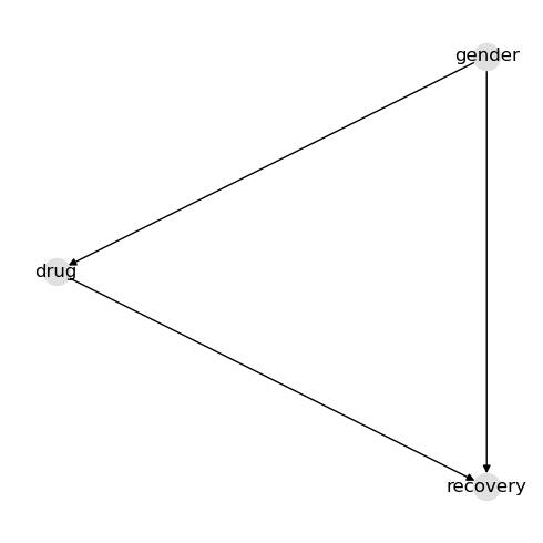
Simply define your structure using a dictionary. The nodes in this graph mean the following.
genderis male or femaledrugis whether the person/patient took the medicationrecoveryis whether the person recovered
In this example, the drug affects recovery. Gender affects both drug usage and recovery. These made-up relationships form a simple confounder example.
[1]:
d = {
    "nodes": ["drug", "gender", "recovery"],
    "edges": [["gender", "drug"], ["gender", "recovery"], ["drug", "recovery"]],
}
[2]:
from help.viz import get_graph_layout
from pybbn.associational import dict_to_graph
import networkx as nx
import matplotlib.pyplot as plt

fig, ax = plt.subplots(figsize=(5, 5))

g = dict_to_graph(d)
pos = get_graph_layout(g, seed=37)
nx.draw(g, pos=pos, with_labels=True, node_color="#e0e0e0")

fig.tight_layout()
1.1.2. Create the parameters, CPTs
The variables in the running examples are binary (they each have 2 values). The parameters (or local probability models) are conditional probability tables (CPTs). A CPT is defined for each node through dictionaries (inspired by Pandas split and records orientations).
[3]:
p = {
    "gender": {
        "columns": ["gender", "__p__"],
        "data": [["male", 0.51], ["female", 0.49]],
    },
    "drug": {
        "columns": ["gender", "drug", "__p__"],
        "data": [
            ["female", "no", 0.23],
            ["female", "yes", 0.77],
            ["male", "no", 0.76],
            ["male", "yes", 0.24],
        ],
    },
    "recovery": {
        "columns": ["gender", "drug", "recovery", "__p__"],
        "data": [
            ["female", "no", "no", 0.31],
            ["female", "no", "yes", 0.69],
            ["female", "yes", "no", 0.27],
            ["female", "yes", "yes", 0.73],
            ["male", "no", "no", 0.13],
            ["male", "no", "yes", 0.87],
            ["male", "yes", "no", 0.07],
            ["male", "yes", "yes", 0.93],
        ],
    },
}
1.1.3. Create the model
We use the create_reasoning_model() convenience method to create an inference model.
[4]:
from pybbn.factory import create_reasoning_model

model = create_reasoning_model(d, p)
1.2. Associational query
Associational queries are probabilistic queries. Associational queries can be executed with different types of evidence. You can also execute associational queries with a mixture of different types of evidences.
1.2.1. Query without evidence
We can query the model without any evidence as follows. The posteriors come back as Pandas dataframes.
[5]:
q = model.pquery()
[6]:
q["gender"]
[6]:
| gender | __p__ | |
|---|---|---|
| 0 | female | 0.49 |
| 1 | male | 0.51 |
[7]:
q["drug"]
[7]:
| drug | __p__ | |
|---|---|---|
| 0 | no | 0.5003 |
| 1 | yes | 0.4997 |
[8]:
q["recovery"]
[8]:
| recovery | __p__ | |
|---|---|---|
| 0 | no | 0.195764 |
| 1 | yes | 0.804236 |
1.2.2. Query with observation evidence
Arguably, observation evidence is the most common type of evidence. Observation evidence assigns one value a weight of 1 and all other values a weight of 0. We can query the model with observation evidence as follows.
[9]:
evidences = {"gender": model.create_observation_evidences("gender", "male")}

q = model.pquery(evidences=evidences)
[10]:
q["gender"]
[10]:
| gender | __p__ | |
|---|---|---|
| 0 | female | 0.0 |
| 1 | male | 1.0 |
[11]:
q["drug"]
[11]:
| drug | __p__ | |
|---|---|---|
| 0 | no | 0.76 |
| 1 | yes | 0.24 |
[12]:
q["recovery"]
[12]:
| recovery | __p__ | |
|---|---|---|
| 0 | no | 0.1156 |
| 1 | yes | 0.8844 |
1.2.3. Query with observation evidence, shortcut
There is a shortcut version to creating observation evidence to alleviate the verbose approach above.
[13]:
q = model.pquery(evidences=model.e({"gender": "male"}))
[14]:
q["gender"]
[14]:
| gender | __p__ | |
|---|---|---|
| 0 | female | 0.0 |
| 1 | male | 1.0 |
[15]:
q["drug"]
[15]:
| drug | __p__ | |
|---|---|---|
| 0 | no | 0.76 |
| 1 | yes | 0.24 |
[16]:
q["recovery"]
[16]:
| recovery | __p__ | |
|---|---|---|
| 0 | no | 0.1156 |
| 1 | yes | 0.8844 |
1.2.4. Exact joint, conditional, and evidence queries
When you need richer exact associational outputs, jquery() returns an exact joint posterior, condquery() returns an exact conditional table, and pevidence() returns the exact probability of a supplied evidence set. Set easy=True when you want the tabular Pandas representation.
[17]:
joint = model.jquery(["drug", "recovery"], evidences=model.e({"gender": "male"}), easy=True)
joint
[17]:
| drug | recovery | __p__ | |
|---|---|---|---|
| 0 | no | no | 0.0988 |
| 1 | no | yes | 0.6612 |
| 2 | yes | no | 0.0168 |
| 3 | yes | yes | 0.2232 |
[18]:
conditional = model.condquery(
    "recovery", ["drug"], evidences=model.e({"gender": "male"}), easy=True
)
conditional
[18]:
| recovery | drug | __p__ | |
|---|---|---|---|
| 0 | no | no | 0.13 |
| 1 | no | yes | 0.07 |
| 2 | yes | no | 0.87 |
| 3 | yes | yes | 0.93 |
[19]:
model.pevidence(model.e({"gender": "male", "drug": "yes", "recovery": "yes"}))
[19]:
0.113832
1.2.5. Query with finding evidence
Finding evidence can only be either \(\{0, 1\}\) and generalizes observation evidence. At least one value must be set to 1, however (or there will be a division by zero issue). The difference with observation evidence is that finding evidence can have multiple values set to 1.
[20]:
evidences = {"gender": model.create_finding_evidences("gender", [1, 0], ["male", "female"])}

q = model.pquery(evidences=evidences)
[21]:
q["gender"]
[21]:
| gender | __p__ | |
|---|---|---|
| 0 | female | 0.0 |
| 1 | male | 1.0 |
[22]:
q["drug"]
[22]:
| drug | __p__ | |
|---|---|---|
| 0 | no | 0.76 |
| 1 | yes | 0.24 |
[23]:
q["recovery"]
[23]:
| recovery | __p__ | |
|---|---|---|
| 0 | no | 0.1156 |
| 1 | yes | 0.8844 |
1.2.6. Query with virtual evidence
Virtual evidence is the most general form of evidence (generalizing both observational and finding evidence types). Virtual evidence has all values in the range \([0, 1]\).
[24]:
evidences = {"gender": model.create_virtual_evidences("gender", [0.01, 0.99], ["male", "female"])}

q = model.pquery(evidences=evidences)
[25]:
q["gender"]
[25]:
| gender | __p__ | |
|---|---|---|
| 0 | female | 0.989596 |
| 1 | male | 0.010404 |
[26]:
q["drug"]
[26]:
| drug | __p__ | |
|---|---|---|
| 0 | no | 0.235514 |
| 1 | yes | 0.764486 |
[27]:
q["recovery"]
[27]:
| recovery | __p__ | |
|---|---|---|
| 0 | no | 0.277498 |
| 1 | yes | 0.722502 |
1.2.7. Query with mixed types of evidence
Here, we show how to issue an associational query with mixed types of evidences.
[28]:
evidences = {
    "gender": model.create_observation_evidences("gender", "male"),
    "drug": model.create_virtual_evidences("drug", [0.60, 0.40], ["yes", "no"]),
}
q = model.pquery(evidences=evidences)
[29]:
q["gender"]
[29]:
| gender | __p__ | |
|---|---|---|
| 0 | female | 0.0 |
| 1 | male | 1.0 |
[30]:
q["drug"]
[30]:
| drug | __p__ | |
|---|---|---|
| 0 | no | 0.678571 |
| 1 | yes | 0.321429 |
[31]:
q["recovery"]
[31]:
| recovery | __p__ | |
|---|---|---|
| 0 | no | 0.110714 |
| 1 | yes | 0.889286 |
1.3. Interventional query
To estimate the causal effects, we can apply the do operator [PGJ16]. For brevity, in the running example, denote the following.
\(G\) is gender
\(D\) is drug
\(R\) is recovery
The (backdoor) adjustment formula is defined as follows.
\(P(R=r|\mathrm{do}(D=d)) = P(R=r|D=d, G=g) P(G=g)\)
We can estimate the causal effects separately.
\(P(R=\mathrm{yes}|\mathrm{do}(D=\mathrm{yes})) = P(R=\mathrm{yes}|D=\mathrm{yes}, G=g) P(G=g)\)
\(P(R=\mathrm{yes}|\mathrm{do}(D=\mathrm{no})) = P(R=\mathrm{yes}|D=\mathrm{no}, G=g) P(G=g)\)
The average causal effect (ACE) can then be computed as follows.
\(\mathrm{ACE} = P(R=\mathrm{yes}|\mathrm{do}(D=\mathrm{yes})) - P(R=\mathrm{yes}|\mathrm{do}(D=\mathrm{no}))\)
[32]:
p_yes = model.iquery(Y=["recovery"], y=["yes"], X=["drug"], x=["yes"])
p_yes
[32]:
recovery    0.832
dtype: float64
[33]:
p_no = model.iquery(Y=["recovery"], y=["yes"], X=["drug"], x=["no"])
p_no
[33]:
recovery    0.7818
dtype: float64
The interpretation of the result below is that taking the drug causally increases the chance of recovery by about 5.02 percentage points.
[34]:
p_yes["recovery"] - p_no["recovery"]
[34]:
np.float64(0.05020000000000013)
1.3.1. Richer exact interventional queries
When you need more than a single event probability under an intervention, compile the intervened model once with intervene() and then reuse the exact associational query methods on that intervened model.
[35]:
treated = model.intervene({"drug": "yes"})
treated.jquery(["gender", "recovery"], easy=True)
[35]:
| gender | recovery | __p__ | |
|---|---|---|---|
| 0 | female | no | 0.1323 |
| 1 | female | yes | 0.3577 |
| 2 | male | no | 0.0357 |
| 3 | male | yes | 0.4743 |
[36]:
treated.condquery("recovery", ["gender"], easy=True)
[36]:
| recovery | gender | __p__ | |
|---|---|---|---|
| 0 | no | female | 0.27 |
| 1 | no | male | 0.07 |
| 2 | yes | female | 0.73 |
| 3 | yes | male | 0.93 |
[37]:
treated.pevidence(treated.e({"gender": "male", "recovery": "yes"}))
[37]:
0.47430000000000005
1.4. Counterfactual query
In this example, we want to compute the counterfactual: Given that a male patient did not take the drug and did not recover, what would the probability of recovery be had the patient taken the drug?
The evidence is that the patient is male, did not take the drug, and did not recover. This evidence is factual; it is what actually happened.
\(G=\mathrm{male}\)
\(D=\mathrm{no}\)
\(R=\mathrm{no}\)
The hypothetical intervention is had the patient taken the drug. This is the counterfactual.
\(D^*=\mathrm{yes}\)
The probability of interest is recovery in the counterfactual.
\(P_{d'}(R | G=g, D=d)\)
[38]:
Y = "recovery"
e = {"gender": "male", "drug": "no", "recovery": "no"}
h = {"drug": "yes"}
The probability of recovery for the counterfactual is 46.15%.
[39]:
model.cquery(Y, e, h)
[39]:
| recovery | __p__ | |
|---|---|---|
| 0 | no | 0.538462 |
| 1 | yes | 0.461538 |
1.4.1. Richer exact counterfactual queries
When you need more than a single counterfactual marginal, cpquery(), cjquery(), ccondquery(), and cpevidence() expose the richer exact query shapes while still conditioning on the factual evidence e.
[40]:
model.cpquery(nodes=["gender", "recovery"], e=e, h=h, easy=True)
[40]:
{'gender':    gender  __p__
 0  female    0.0
 1    male    1.0,
 'recovery':   recovery     __p__
 0       no  0.538462
 1      yes  0.461538}
[41]:
model.cjquery(["gender", "recovery"], e=e, h=h, easy=True)
[41]:
| gender | recovery | __p__ | |
|---|---|---|---|
| 0 | female | no | 0.000000 |
| 1 | female | yes | 0.000000 |
| 2 | male | no | 0.538462 |
| 3 | male | yes | 0.461538 |
[42]:
e2 = {"drug": "no", "recovery": "no"}
model.ccondquery("recovery", ["gender"], e=e2, h=h, easy=True)
[42]:
| recovery | gender | __p__ | |
|---|---|---|---|
| 0 | no | female | 0.870968 |
| 1 | no | male | 0.538462 |
| 2 | yes | female | 0.129032 |
| 3 | yes | male | 0.461538 |
[43]:
model.cpevidence({"recovery": "yes"}, e=e, h=h)
[43]:
0.4615384615384615
1.5. Graphical query
Below are some examples of graphical queries.
1.5.1. d-separation and conditional independence
Querying if two nodes are d-separated is possible [Pea18].
[44]:
model.is_d_separated("drug", "recovery")
[44]:
False
[45]:
model.is_d_separated("drug", "recovery", {"gender"})
[45]:
False
1.5.2. Confounders and backdoors
We can query for the minimal set of confounders between two nodes [PGJ16].
[46]:
model.get_minimal_confounders("drug", "recovery")
[46]:
['gender']
1.5.3. Mediators and frontdoors
We can query for the minimal set of mediators between two nodes [PGJ16]. In this running example, there are no frontdoors.
[47]:
model.get_minimal_mediators("drug", "recovery")
[47]:
[]
1.6. Data sampling
Sampling uses compiled ancestral draws [Hen88]. If evidence is provided, then likelihood weighting is used and rows are resampled back into a standard DataFrame.
[48]:
sample_df = model.sample(max_samples=1_000)
sample_df.shape
[48]:
(1000, 3)
[49]:
sample_df.head()
[49]:
| gender | drug | recovery | |
|---|---|---|---|
| 0 | female | no | yes |
| 1 | female | yes | no |
| 2 | male | no | yes |
| 3 | female | yes | yes |
| 4 | male | no | yes |
1.7. Serde
Saving and loading the model is easy.
1.7.1. Serialization
To persist the model, use model_to_dict() to create a Python dictionary and then serialize the dictionary as JSON data.
[50]:
import json
import tempfile
from pybbn.serde import model_to_dict

data1 = model_to_dict(model)

with tempfile.NamedTemporaryFile(mode="w", delete=False) as fp:
    json.dump(data1, fp)

    file_path = fp.name

print(f"{file_path=}")
file_path='/tmp/tmpo2m_8r4v'
1.7.2. Deserialization
To restore the model, use the json module to deserialize the dictionary, and then use dict_to_model() to recreate the model.
[51]:
from pybbn.serde import dict_to_model

with open(file_path, "r") as fp:
    data2 = json.load(fp)

model2 = dict_to_model(data2)
[52]:
q = model2.pquery()
[53]:
q["gender"]
[53]:
| gender | __p__ | |
|---|---|---|
| 0 | female | 0.49 |
| 1 | male | 0.51 |
[54]:
q["drug"]
[54]:
| drug | __p__ | |
|---|---|---|
| 0 | no | 0.5003 |
| 1 | yes | 0.4997 |
[55]:
q["recovery"]
[55]:
| recovery | __p__ | |
|---|---|---|
| 0 | no | 0.195764 |
| 1 | yes | 0.804236 |